Air Density Estimation Tool for Japan

Overview

Japan’s dense meteorological observation network is a valuable independent reference for wind-resource work. Wind speed and direction are the obvious variables, but pressure, temperature and humidity are also important because they determine air density—and therefore the kinetic power available in the wind.

I developed this project to answer a practical early-stage question:

Can I estimate a representative long-term air density for a location in Japan using only its latitude and elevation?

The result is an end-to-end Python workflow that:

discovers observation stations from the Japan Meteorological Agency (JMA) station maps;
collects monthly pressure, temperature and humidity observations;
calculates humid-air density for every station;
develops a regression model that estimates long-term mean air density from elevation and latitude; and
implements the model as an interactive tool for estimating air density at any location in Japan.

The estimator provides a long-term climatological value, and it is intended for preliminary wind-resource screening, measurement planning and engineering reasonableness checks.

Try the air-density estimator

Enter the latitude and elevation above mean sea level for a location in Japan. The calculator applies the fitted 2006-2025 station-mean regression model described later on this page.

Estimated long-term mean 1.215 kg/m³ Elevation: 20 m MSL | -0.8% vs 1.225 kg/m³

Using the result

The tool returns the modelled 2006-2025 long-term mean air density at the entered elevation in kg/m³. It can support early-stage site comparisons and provide an initial assumption before local measurements are available. It does not replace simultaneous pressure, temperature and humidity measurements for turbine power-performance testing or bankable energy-yield analysis.

Workflow

JMA station maps
      ↓
Station catalogue: ID, type, latitude, longitude, elevation
      ↓
Monthly pressure, temperature and humidity: 2006–2025
      ↓
Humid-air density for each station-month
      ↓
Long-term station means
      ↓
Elevation model + latitude residual correction
      ↓
Interactive latitude/elevation estimator

1. Building the station catalogue

JMA’s historical weather-data selector uses regional image maps. The underlying HTML contains the identifiers and metadata needed to turn the visual map into a structured station catalogue.

The two key identifiers are:

prec_no: JMA’s regional code; and
block_no: the observation-station code.

The station markup also provides the station name, latitude, longitude and elevation. The notebook follows the station-discovery approach described in Sako-san’s post, “How to Obtain Weather Data at Locations in Japan”, then extends it with geographic filtering, station classification and reusable metadata fields.

import re
import time
from urllib.parse import urljoin

import pandas as pd
import requests
from bs4 import BeautifulSoup

BASE = "https://www.data.jma.go.jp/stats/etrn"

session = requests.Session()
session.headers.update({
    "User-Agent": "JMA research project; contact: replace-with-your-email"
})


def soup_for(url):
    response = session.get(url, timeout=30)
    response.raise_for_status()
    response.encoding = "utf-8"
    return BeautifulSoup(response.text, "html.parser")


def build_station_catalogue(delay=1.0):
    root_url = (
        f"{BASE}/select/prefecture00.php"
        "?prec_no=&block_no=&year=&month=&day=&view="
    )
    root = soup_for(root_url)
    stations = []

    for region in root.select("area[href]"):
        href = region.get("href", "")
        match = re.search(r"prec_no=(\d+)", href)
        if not match:
            continue

        prec_no = match.group(1)
        region_page = soup_for(urljoin(root_url, href))

        for area in region_page.select("area[onmouseover]"):
            args = area["onmouseover"].split("'")
            if len(args) < 18:
                continue

            block_no = args[3]
            stations.append({
                "prec_no": prec_no,
                "block_no": block_no,
                "station": args[5],
                "station_type": "s1" if len(block_no) == 5 else "a1",
                "latitude": float(args[9]) + float(args[11]) / 60,
                "longitude": float(args[13]) + float(args[15]) / 60,
                "elevation_m": float(args[17]),
            })

        time.sleep(delay)

    stations = pd.DataFrame(stations).drop_duplicates()
    return stations[
        stations["latitude"].between(20, 46)
        & stations["longitude"].between(120, 150)
    ].reset_index(drop=True)

The saved notebook run retained 1,677 station records after coordinate filtering. This catalogue becomes the common spatial index for every later step.

2. Collecting JMA monthly observations

The density calculation requires local pressure, mean temperature and relative humidity. These variables are available on the richer JMA s1 surface-station pages. A monthly request is defined by the station keys and year:

monthly_s1.php?prec_no={region}&block_no={station}&year={year}

Each response contains up to twelve monthly rows. The parser checks the table width before assigning names, selects only the fields needed for density, converts JMA symbols to missing values and attaches the station metadata.

from io import StringIO

import numpy as np


def fetch_monthly_s1(station, year):
    url = (
        f"{BASE}/view/monthly_s1.php"
        f"?prec_no={station['prec_no']}"
        f"&block_no={station['block_no']}"
        f"&year={year}&month=&day=&view="
    )

    response = session.get(url, timeout=30)
    response.raise_for_status()
    response.encoding = "utf-8"
    raw_table = pd.read_html(StringIO(response.text))[0]

    # The current 'main elements' s1 table contains 28 columns.
    if raw_table.shape[1] != 28:
        raise ValueError(
            f"Unexpected JMA schema for {station['block_no']} in {year}: "
            f"{raw_table.shape[1]} columns"
        )

    monthly = pd.DataFrame({
        "month": raw_table.iloc[:12, 0],
        "local_pressure_hpa": raw_table.iloc[:12, 1],
        "mean_temperature_c": raw_table.iloc[:12, 7],
        "mean_relative_humidity_pct": raw_table.iloc[:12, 12],
    })

    for column in monthly.columns:
        monthly[column] = pd.to_numeric(monthly[column], errors="coerce")

    monthly["year"] = year
    monthly["station"] = station["station"]
    monthly["prec_no"] = station["prec_no"]
    monthly["block_no"] = station["block_no"]
    monthly["latitude"] = station["latitude"]
    monthly["longitude"] = station["longitude"]
    monthly["elevation_m"] = station["elevation_m"]

    return monthly.dropna(subset=[
        "local_pressure_hpa",
        "mean_temperature_c",
        "mean_relative_humidity_pct",
    ])

The collection loop is deliberately sequential. Raw responses are cached locally, completed station-years are recorded in a manifest, and failed or changed schemas stop the run rather than being silently accepted.

monthly_frames = []
s1_stations = stations[stations["station_type"] == "s1"]

for station in s1_stations.to_dict("records"):
    for year in range(2006, 2026):
        try:
            monthly_frames.append(fetch_monthly_s1(station, year))
        except Exception as exc:
            record_failure(station, year, exc)
        time.sleep(1.0)

monthly = pd.concat(monthly_frames, ignore_index=True)
monthly.to_csv("jma_monthly_2006_2025.csv", index=False)

JMA asks users to avoid excessive automated access. In practice, I use delays, caching, limited retries and resumable jobs, and I do not parallelise requests against the public service.

Resulting analysis dataset

Item	Result
Period	2006–2025
Surface stations used	153
Station-years requested	3,060
Station-month rows	36,720
Density inputs	Local pressure, temperature, relative humidity

3. Calculating humid-air density

Air density is calculated for each station-month before aggregation. For moist air:

ρ = (p − e) / (R_dT) + e / (R_vT)

where p is local pressure, e is water-vapour partial pressure, T is absolute temperature, and R_d and R_v are the specific gas constants for dry air and water vapour.

def humid_air_density(temp_c, pressure_hpa, rh_pct):
    temp_c = np.asarray(temp_c, dtype=float)
    pressure_hpa = np.asarray(pressure_hpa, dtype=float)
    rh_pct = np.asarray(rh_pct, dtype=float)

    temp_k = temp_c + 273.15
    pressure_pa = pressure_hpa * 100

    # Tetens-family saturation-vapour-pressure approximation
    saturation_hpa = 6.1078 * np.exp(
        17.27 * temp_c / (237.5 + temp_c)
    )
    vapour_pa = (rh_pct / 100) * saturation_hpa * 100

    r_dry = 287.058
    r_vapour = 461.495

    return (
        (pressure_pa - vapour_pa) / (r_dry * temp_k)
        + vapour_pa / (r_vapour * temp_k)
    )


monthly["density_kg_m3"] = humid_air_density(
    monthly["mean_temperature_c"],
    monthly["local_pressure_hpa"],
    monthly["mean_relative_humidity_pct"],
)

Monthly densities are averaged into station-year means and then into a 2006–2025 long-term mean for each station:

annual = (
    monthly.groupby([
        "station", "year", "latitude", "longitude", "elevation_m"
    ])["density_kg_m3"]
    .mean()
    .rename("annual_density_kg_m3")
    .reset_index()
)

long_term = (
    annual.groupby([
        "station", "latitude", "longitude", "elevation_m"
    ])["annual_density_kg_m3"]
    .mean()
    .rename("density_kg_m3")
    .reset_index()
)

4. Developing the regression model

Stage 1: elevation

Elevation captures the primary pressure effect. The first linear regression relates long-term density to station elevation:

ρ̂_elevation = 1.21746 − 0.000110927z

where z is elevation in metres. Within the fitted station range, the coefficient corresponds to approximately 0.0111 kg/m³ less density per 100 m of elevation.

The elevation-only model produces R² = 0.5775. Elevation explains the dominant pressure trend, but the remaining error has a clear geographic pattern.

Stage 2: latitude correction

The residual from the elevation model is regressed against latitude:

residual = −0.14008 + 0.00392261φ

where φ is latitude in decimal degrees north. Latitude acts as a compact proxy for Japan’s broad north–south temperature gradient.

def fit_linear(x, y):
    design = np.column_stack([np.ones(len(x)), x])
    coefficients, *_ = np.linalg.lstsq(design, y, rcond=None)
    prediction = design @ coefficients
    r2 = 1 - np.sum((y - prediction) ** 2) / np.sum((y - y.mean()) ** 2)
    return coefficients[0], coefficients[1], prediction, r2


elevation = long_term["elevation_m"].to_numpy()
latitude = long_term["latitude"].to_numpy()
density = long_term["density_kg_m3"].to_numpy()

# Stage 1: density from elevation
elev_intercept, elev_slope, elev_prediction, elev_r2 = fit_linear(
    elevation, density
)

# Stage 2: elevation residual from latitude
residual = density - elev_prediction
lat_intercept, lat_slope, residual_prediction, residual_r2 = fit_linear(
    latitude, residual
)

final_prediction = elev_prediction + residual_prediction
final_r2 = 1 - np.sum((density - final_prediction) ** 2) / np.sum(
    (density - density.mean()) ** 2
)

Regression result

Combining the elevation model and latitude correction gives the final screening equation:

ρ̂ = 1.07738 + 0.00392261φ − 0.000110927z

Model	Inputs	R²
Stage 1	Elevation	0.5775
Final model	Elevation + latitude correction	0.9824

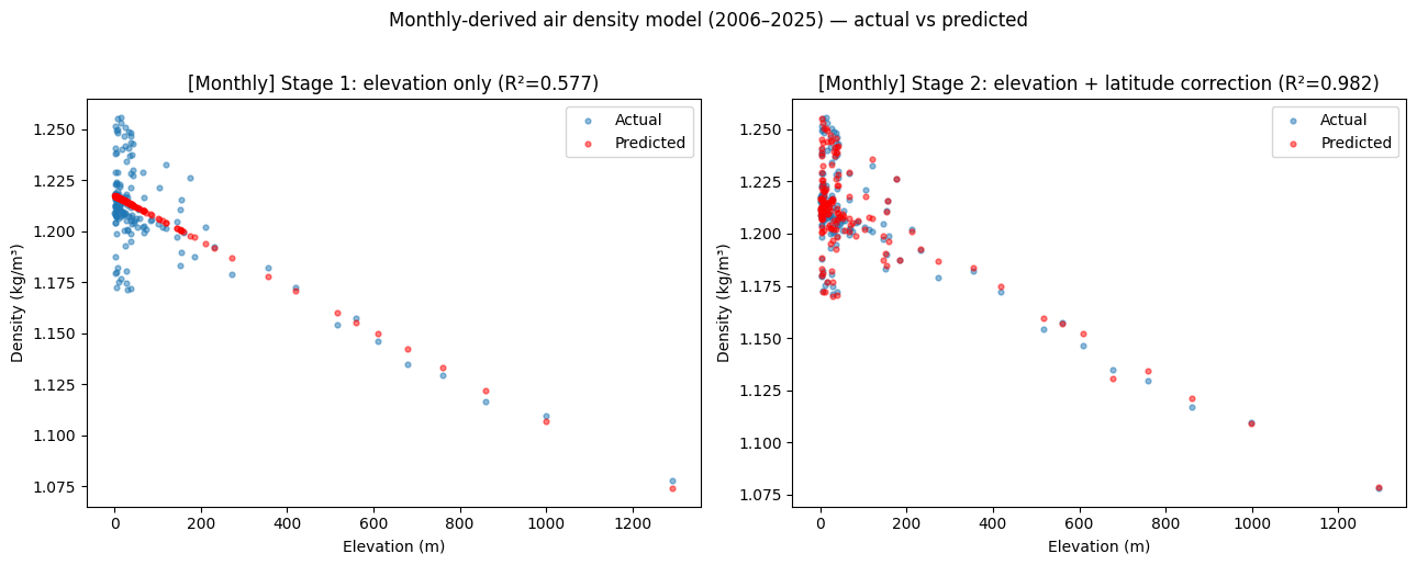
Calculated and modelled long-term air density across JMA surface stations. The elevation-only result is shown on the left; the latitude-corrected result is shown on the right.

Monthly-derived long-term air density for 153 JMA surface stations, 2006–2025. Source: author’s calculations based on Japan Meteorological Agency observations; the source data were processed and modelled by the author.

Method note: station counts, monthly row counts and fitted coefficients are saved-run results from the project notebook. JMA pages, schemas and observations may change. The chart and regression model are the author’s derived work based on JMA observations.